Factor analysis. Factor analysis methods Factor analysis by chain substitution method
Statistica 6 q. Preparation of correlation matrix for factor analysis q. Creating a matrix for factor analysis q. Factor analysis q. Isolation of factor loadings q. Construction of a factor diagram
 Preparing a correlation matrix for factor analysis in the Statistica program Since our ranks are ordinal scales, two coefficients will be adequate for this type of scale: Spearman and Kendall. We will consider Kendall, since he is more accurate. We enter our raw data into the Statistica program


 We received a factor matrix calculated by the Kendall coefficient, since it is this that is adequate for our data, which are order scales.
 Creating a matrix for calculating FA Now you need to create a matrix of such a structure that Statistica can use it to carry out factor analysis. It is necessary that the matrix, in addition to the values of correlations between variables, include 4 more rows below them: 1) average values of ranks, 2) standard deviations of ranks, 3) number of evaluated objects and 4) type of matrix. Click Analysis and select Basic statistics and tables


 As a result, we received a correlation matrix for FA that Statistica can read. However, the correlation analysis here was carried out by the Pearson coefficient. Therefore, this correlation matrix (5 x 5) needs to be replaced with the one we calculated using the Kendall coefficient (copy and paste).
 As can be seen, the Kendall correlation values differ from the Pearson values. This is because our ranks are order scales for which the use of the Pearson coefficient is inadequate. Now we can proceed to factor analysis.

 Variables → select all 5 variables Var 1 Var 5 → in the Data file field set Correlation matrix → OK
 Max. We set the number of factors to 5 (since we have only 5 variables) → select the Centroid method (was developed by Thurstone and implements a geometric approach to FA) → OK
 The program identified 2 factors. To view factor loadings, click the Factor loadings button. To construct a factor diagram, click on the 2 M loading plot.


 Statgraphics Centurion q. Factor analysis q. Isolation of factor loadings q. Constructing a factor diagram q. Building an object diagram
 The program does not provide the ability to create your own correlation matrix, so we start immediately with an analysis of our ranks. We enter our ranks and select Analyze → Variable Data → Multivariate Methods → Factor Analysis

 As a result, the program allocated us 2 factors with a level of explained variance of 82.468%. This means that these factors explain 82.468% (almost 4/5) of all our information across the five variables.
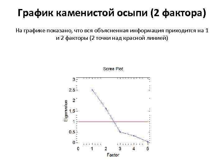 Scree plot (2 factors) The graph shows that all the information explained is in factors 1 and 2 (2 points above the red line)
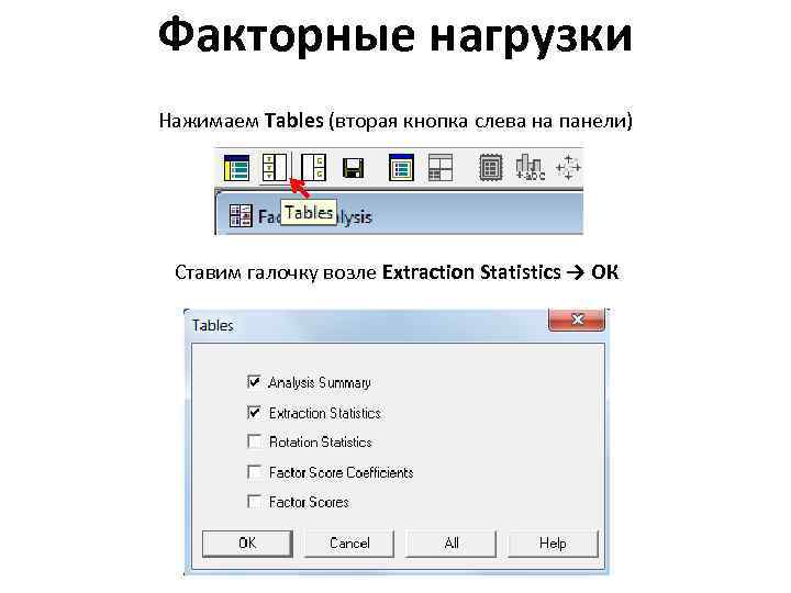 Factor loadings Click Tables (second button from the left on the panel) Check the box next to Extraction Statistics → OK
 As you can see, the factor loadings at the tenth level differ from those we obtained by manual calculation and in Statistica. This is explained by the fact that Statgraphics cannot include its own correlation matrix and the program always considers the Pearson coefficient, which is not adequate for data on order scales.
 Factor chart Click Graphs (third button from the left on the panel) Check the box next to 2 D Factor Plot (if we had more than 2 factors, we would check the box next to 3 D Factor Plot to get a three-dimensional graph) → OK
 We obtained a factor matrix after rotation. Segments (projections of points formed by factor loadings) 2 and 5 are located close to the y-axis (tend to 0) and are distant from the x-axis. This means that the x-axis coordinates of these points (which corresponds to the first factor) are represented by low values (0, 6). Therefore, scales 2 and 5 represent 1 factor. By the same principle, segment 1 indicates that scales 1, 3 and 4 represent factor 2.
 Object diagram Click Graphs (third button from the left on the panel) Check the box next to 2 D Scatterplot (if we had more than 2 factors, we would check the box next to 3 D Scatterplot to get a three-dimensional graph) → OK
Factor analysis is a statistical method that is used when processing large amounts of experimental data. The objectives of factor analysis are: reducing the number of variables (data reduction) and determining the structure of relationships between variables, i.e. classification of variables, so factor analysis is used as a data reduction method or as a structural classification method.
An important difference between factor analysis and all the methods described above is that it cannot be used to process primary, or, as they say, “raw” experimental data, i.e. obtained directly from the examination of subjects. The material for factor analysis is correlations, or more precisely, Pearson correlation coefficients, which are calculated between the variables (i.e. psychological characteristics) included in the survey. In other words, correlation matrices, or, as they are otherwise called, intercorrelation matrices, are subjected to factor analysis. The column and row names in these matrices are the same because they represent a list of variables included in the analysis. For this reason, intercorrelation matrices are always square, i.e. the number of rows in them is equal to the number of columns, and symmetrical, i.e. symmetrical places relative to the main diagonal have the same correlation coefficients.
The main concept of factor analysis is factor. This is an artificial statistical indicator that arises as a result of special transformations of the table of correlation coefficients between the studied psychological characteristics, or the intercorrelation matrix. The procedure for extracting factors from an intercorrelation matrix is called matrix factorization. As a result of factorization, a different number of factors can be extracted from the correlation matrix, up to a number equal to the number of original variables. However, the factors identified as a result of factorization, as a rule, are unequal in importance. (5)
With the help of identified factors, the interdependence of psychological phenomena is explained. (7)
Most often, as a result of factor analysis, not one, but several factors are determined that differently explain the matrix of intercorrelations of variables. In this case, factors are divided into general, general and individual. General factors are those all factor loadings of which differ significantly from zero (zero loading indicates that this variable is in no way connected with the others and does not have any influence on them in life). General are factors for which some of the factor loadings are different from zero. Single factors are factors in which only one of the loadings differs significantly from zero. (7)
Factor analysis may be appropriate if the following criteria are met.
- 1. It is impossible to factorize qualitative data obtained on a scale of names, for example, such as hair color (black / chestnut / red), etc.
- 2. All variables must be independent, and their distribution must approach normal.
- 3. Relationships between variables should be approximately linear, or at least not clearly curvilinear.
- 4. The initial correlation matrix should contain several correlations with a modulus higher than 0.3. Otherwise, it is quite difficult to extract any factors from the matrix.
- 5. The sample of subjects must be large enough. Expert recommendations vary. The most stringent point of view recommends not using factor analysis if the number of subjects is less than 100, since the standard errors of correlation in this case will be too large.
However, if the factors are well defined (for example, with loadings of 0.7 rather than 0.3), the experimenter needs a smaller sample to isolate them. In addition, if the data obtained are known to be highly reliable (for example, valid tests are used), then data can be analyzed on a smaller number of subjects. (5).
Called factor analysis. The main types of factor analysis are deterministic analysis and stochastic analysis.
Deterministic factor analysis is based on a methodology for studying the influence of such factors, the relationship of which with a general economic indicator is functional. The latter means that the generalizing indicator is either a product, a quotient of division, or an algebraic sum of individual factors.
Stochastic factor analysis is based on a methodology for studying the influence of such factors, the relationship of which with a general economic indicator is probabilistic, otherwise - correlation.
In the presence of a functional relationship with a change in the argument, there is always a corresponding change in the function. If there is a probabilistic relationship, a change in the argument can be combined with several values of the change in the function.
Factor analysis is also divided into straight, otherwise deductive analysis and back(inductive) analysis.
First type of analysis carries out the study of the influence of factors by a deductive method, that is, in the direction from the general to the specific. In reverse factor analysis the influence of factors is studied inductively - in the direction from particular factors to general economic indicators.
Classification of factors influencing the efficiency of an organization
The factors whose influence is studied during the study are classified according to various criteria. First of all, they can be divided into two main types: internal factors, depending on the activity of this, and external factors, independent of this organization.
Internal factors, depending on the magnitude of their impact on, can be divided into major and minor. The main ones include factors related to the use of materials and materials, as well as factors determined by supply and sales activities and some other aspects of the functioning of the organization. The main factors have a fundamental impact on general economic indicators. External factors beyond the control of a given organization are determined by natural-climatic (geographical), socio-economic, and foreign economic conditions.
Depending on the duration of their impact on economic indicators, we can distinguish constant and variable factors. The first type of factors has an impact on economic indicators that is not limited in time. Variable factors affect economic indicators only over a certain period of time.
Factors can be divided into extensive (quantitative) and intensive (qualitative) based on the essence of their influence on economic indicators. So, for example, if the influence of labor factors on the volume of output is studied, then a change in the number of workers will be an extensive factor, and a change in the labor productivity of one worker will be an intensive factor.
Factors influencing economic indicators, according to the degree of their dependence on the will and consciousness of the organization’s employees and other persons, can be divided into objective and subjective factors. Objective factors may include weather conditions and natural disasters that do not depend on human activity. Subjective factors depend entirely on people. The vast majority of factors should be classified as subjective.
Factors can also be divided depending on the scope of their action into factors of unlimited and factors of limited action. The first type of factors operates everywhere, in all sectors of the national economy. The second type of factors influences only within an industry or even a separate organization.
According to their structure, factors are divided into simple and complex. The overwhelming majority of factors are complex, including several components. At the same time, there are also factors that cannot be separated. For example, capital productivity can serve as an example of a complex factor. The number of days the equipment was used during a given period is a simple factor.
According to the nature of the influence on general economic indicators, they are distinguished direct and indirect factors. Thus, a change in products sold, although it has an inverse effect on the amount of profit, should be considered direct factors, that is, a first-order factor. A change in the amount of material costs has an indirect effect on profit, i.e. affects profit not directly, but through cost, which is a first-order factor. Based on this, the level of material costs should be considered a second-order factor, that is, an indirect factor.
Depending on whether it is possible to quantify the influence of a given factor on a general economic indicator, a distinction is made between measurable and unmeasurable factors.
This classification is closely interconnected with the classification of reserves for increasing the efficiency of economic activities of organizations, or, in other words, reserves for improving the analyzed economic indicators.
Factor economic analysis
Those signs that characterize the cause are called factorial, independent. The same signs that characterize the investigation are usually called resultant, dependent.
The set of factor and resultant characteristics that are in the same cause-and-effect relationship is called factor system. There is also the concept of a factor system model. It characterizes the relationship between the resultant characteristic, denoted as y, and the factor characteristics, denoted as . In other words, the factor system model expresses the relationship between general economic indicators and individual factors influencing this indicator. In this case, other economic indicators act as factors, representing the reasons for changes in the general indicator.
Factor system model can be expressed mathematically using the following formula:
Establishing dependencies between generalizing (resulting) and influencing factors is called economic-mathematical modeling.
We study two types of relationships between generalizing indicators and the factors influencing them:
- functional (otherwise - functionally determined, or strictly determined connection.)
- stochastic (probabilistic) connection.
Functional connection- this is a relationship in which each value of a factor (factorial characteristic) corresponds to a completely definite non-random value of a generalizing indicator (resultative characteristic).
Stochastic communication- this is a relationship in which each value of a factor (factor characteristic) corresponds to a set of values of a general indicator (resultative characteristic). Under these conditions, for each value of factor x, the values of the general indicator y form a conditional statistical distribution. As a result, a change in the value of factor x only on average causes a change in the general indicator y.
In accordance with the two types of relationships considered, a distinction is made between methods of deterministic factor analysis and methods of stochastic factor analysis. Consider the following diagram:
Methods used in factor analysis. Scheme No. 2The greatest completeness and depth of analytical research, the greatest accuracy of analysis results is ensured by the use of economic and mathematical research methods.
These methods have a number of advantages over traditional and statistical methods of analysis.
Thus, they provide a more accurate and detailed calculation of the influence of individual factors on changes in the values of economic indicators and also make it possible to solve a number of analytical problems that cannot be done without the use of economic and mathematical methods.
Jae-On Kim, Charles W. Mueller. Factor Analysis: Statistical Methods and Practical Issues (Eleventh Printing, 1986).
PREFACE
This work is a continuation of the book “Introduction to Factor Analysis: What It Is and How to Use It” by Jae-On Kim and Charles W. Mueller, also published in the Quantitative Applications in the Social Sciences series. The latter is an introduction to the method of factor analysis; it answers the reader’s questions: “What is factor analysis used for?” and “What assumptions are made when using this method?”, but do not address the application of factor analysis to specific data. Factor Analysis: Statistical Methods and Practical Issues discusses in more detail specific examples of data analysis, different types of factor analysis, and situations where its use is most useful. The distinction between confirmatory and exploratory factor analysis is discussed here in more detail than in Introduction to Factor Analysis. For example, various criteria for factor rotation are considered. Particularly useful is the discussion of the various forms of oblique rotations and the interpretation of coefficients in factor analysis. Joe. Kim and C.W. Mueller also raise the question of the number of factors appearing in exploratory factor analysis, examine methods for testing hypotheses in confirmatory analysis, and consider the problem of calculating factor values. A dictionary of special terms is offered, as well as answers to questions that most often arise among users of factor analysis, which can prevent them from making many mistakes. The mathematical apparatus is quite modest - only information from matrix algebra is given.
Factor analysis has been used in economic problems in which the presence of highly correlated parameters led to incorrect results in regression analysis. Scientists dealing with socio-political problems have compared all sorts of characteristics of nations with different political and socio-economic characteristics, trying to determine which of them are most important in classifying nations (for example, wealth and numbers); Sociologists defined “friendly groups” by studying groups of people who sympathized with each other (and not with other individuals). Psychologists have used factor analysis to determine how people perceive various "stimuli" and classify people into groups corresponding to different responses, and publishers have used factor analysis to study ways to associate individual elements of language.
According to the authors, their work does not cover all aspects of factor analysis, since it is constantly evolving. However, if the reader gains a sufficient understanding of how this method can be used, then the authors can be considered to have completed their task.
E. M. Aslaner, series editor
To analyze the variability of a trait under the influence of controlled variables, the dispersion method is used.
To study the relationship between values - the factorial method. Let's take a closer look at the analytical tools: factorial, dispersion and two-factor dispersion methods for assessing variability.
Analysis of Variance in Excel
Conventionally, the goal of the dispersion method can be formulated as follows: to isolate 3 partial variations from the general variability of the parameter:
- 1 – determined by the action of each of the studied values;
- 2 – dictated by the relationship between the studied values;
- 3 – random, dictated by all unaccounted for circumstances.
In Microsoft Excel, analysis of variance can be performed using the “Data Analysis” tool (the “Data” tab - “Analysis”). This is a spreadsheet add-on. If the add-in is not available, you need to open Excel Options and enable the Analysis setting.
The work begins with the design of the table. Rules:
- Each column should contain the values of one factor under study.
- Arrange the columns in ascending/descending order of the value of the parameter being studied.
Let's look at variance analysis in Excel using an example.
The company's psychologist analyzed the behavior strategies of employees in a conflict situation using a special technique. It is assumed that behavior is influenced by the level of education (1 – secondary, 2 – specialized secondary, 3 – higher).
Let's enter the data into an Excel table:


The significant parameter is filled in yellow. Since the P-Value between groups is greater than 1, Fisher's test cannot be considered significant. Consequently, behavior in a conflict situation does not depend on the level of education.
Factor analysis in Excel: example
Factorial analysis is a multidimensional analysis of relationships between the values of variables. Using this method you can solve the most important problems:
- comprehensively describe the object being measured (and succinctly, compactly);
- identify hidden variable values that determine the presence of linear statistical correlations;
- classify variables (identify relationships between them);
- reduce the number of required variables.
Let's look at an example of factor analysis. Let's say we know the sales of some goods over the last 4 months. It is necessary to analyze which titles are in demand and which are not.


Now you can clearly see which product sales are generating the main growth.
Two-way ANOVA in Excel
Shows how two factors influence the change in the value of a random variable. Let's look at two-factor analysis of variance in Excel using an example.
Task. A group of men and women were presented with sounds of different volumes: 1 – 10 dB, 2 – 30 dB, 3 – 50 dB. Response times were recorded in milliseconds. It is necessary to determine whether gender influences the response; Does volume affect response?
 (1 ratings, on average: 5,00 out of 5)